在神经网络训练过程当中，如果是利用jupyter-notebook来进行代码编写的话，可能断开之后不会看到输出的结果。利用logging模块可以将内容同时输出到文件和终端，首先定义构造logger的函数内容如下：

1
2
3
4
5
6
7
8
9
10
11
12
13
14
15
16
17
18
19
20
21

import logging

def get_logger(filename, verbosity=1, name=None):
    level_dict = {0: logging.DEBUG, 1: logging.INFO, 2: logging.WARNING}
    formatter = logging.Formatter(
        "[%(asctime)s][%(filename)s][line:%(lineno)d][%(levelname)s] %(message)s"
    )
    logger = logging.getLogger(name)
    logger.setLevel(level_dict[verbosity])

    # Output to file
    fh = logging.FileHandler(filename, "w")
    fh.setFormatter(formatter)
    logger.addHandler(fh)

    # Output to terminal
    sh = logging.StreamHandler()
    sh.setFormatter(formatter)
    logger.addHandler(sh)

    return logger

之后在训练流程当中通过以上的函数生成logger，再采用info方法进行保存就可以了：

1
2
3
4
5
6
7
8
9
10

logger = get_logger('./train.log')

logger.info('start training!')
for epoch in range(EPOCHS):
    ...
    loss = ...
    acc = ...
    logger.info('Epoch:[{}/{}]\t loss={:.5f}\t acc={:.3f}'.format(epoch, EPOCHS, loss, acc))
    ...
logger.info('finish training!')

Introduction

正常的分布式训练方法会传递所有的梯度，但是实际上，可能有超过99%的梯度交换都是无关紧要的，所以可以通过只传送重要的梯度来减少在深度学习的分布式训练当中通信带宽。DGC方法通过稀疏更新来只传递重要的梯度，同时利用Momentum Correction，Gradient Clipping等方法来预防不收敛的情形，保证分布式训练不会影响最终的模型准确性。

Deep Gradient Compression

Gradient Sparsification

那么如何来衡量一个梯度的重要性呢，显然如果一个网络节点的梯度大小绝对值更大的话，它会带来的权重更新就会更大，那么对于整个网络的变化趋势而言，就是更为重要的。在DGC方法当中，认为绝对值大小超过某一阈值的梯度为重要的梯度。但是如果只传递此类重要梯度的话，和损失函数的优化目标会存在一定程度上的差距，所以出于减少信息损失的考虑，把剩下不重要的梯度在本地进行累积，那么只要时间足够，最终累积梯度就会超过所设定的阈值，进行梯度交换。

由于仅仅是数值较大的梯度进行了立即传递，较小的梯度在本地进行累积更新，所以能够极大减少每个step交换梯度所需要的通信带宽。那么需要考虑的一点是这种本地梯度累积的方法是否会对于优化目标产生影响，计$f(\cdot)$为损失函数，可以首先分析一个step的更新公式如下：

$w_{t+1}^{(i)} = w_{t}^{(i)}- \eta \frac{1}{Nb}\sum_{k=1}^N \sum_{x\in \mathcal{B}_{k,t}}\nabla^{(i)}f(x,w_t)$

如果在本地进行梯度累积，那么假设在经历过$T$个step之后才进行梯度交换，那么更新公式可以修改为如下形式：

$\begin{aligned} w_{t+T}^{(i)} &= w_{t}^{(i)}- \eta \frac{1}{Nb}\sum_{k=1}^N \sum_{\tau= 0}^{T-1}\sum_{x\in \mathcal{B}_{k,t}}\nabla^{(i)}f(x,w_{t+\tau}) \\ &= w_{t}^{(i)} - \eta T \frac{1}{NbT}\sum_{k=1}^N \left(\sum_{\tau= 0}^{T-1}\sum_{x\in \mathcal{B}_{k,t}}\nabla^{(i)}f(x,w_{t+\tau})\right) \end{aligned}$

那么如上式所示，可以发现当针对于$T$大小进行学习率缩放之后，在分子分母的$T$可以消去，于是总体可以看成是人为的将batch大小从$Nb$提升到了$NbT$。所以直观上本地梯度累积的方法可以看成是随着更新时间区间的拉长来增大训练batch的大小，同时对于学习率进行同比例缩放，并不会影响最终的优化目标。

Momentum Correction

如果直接针对于普通的SGD采用以上的DGC方法，那么先让当更新十分稀疏，即间隔区间长度$T$很大的时候，可能会影响网络的收敛。所以又提出了Momentum Correction和Local Gradient的方法来缓解对于收敛性质的伤害。

最普通的动量方法如下所示，其中$m$的值即为动量。

$u_{t+1} = mu_t + \sum_{k=1}^N \nabla_{k,t},\quad w_{t+1} = w_t - \eta u_t$

事实上最终进行本地的梯度累积和更新都是利用左侧的$u_t$来代替原始梯度$\nabla_t$的，于是可以得到参数更新的表达式如下，假设稀疏更新的时间间隔为$T$。

$\begin{aligned} w_{t+T} ^{(i)} &= w_t^{(i)} - \eta\sum_{k=1}^N\left( \sum_{\tau=0}^{T-1}u_t \right) \\ &= w_t^{(i)} - \eta\sum_{k=1}^N\left[ \left(\sum_{\tau=0}^{T-1}m^\tau\right)\nabla_{k,t}^{(i)}+ \left(\sum_{\tau=0}^{T-2}m^\tau\right)\nabla_{k,t+1}^{(i)} +\ldots\right] \end{aligned}$

对比没有动量修正的更新方法如下：

$\begin{aligned} w_{t+T} ^{(i)} &= w_t^{(i)} - \eta\sum_{k=1}^N\left[\nabla_{k,t}^{(i)}+ \nabla_{k,t+1}^{(i)} +\ldots\right] \end{aligned}$

可以发现实际上缺少了$\sum_{\tau=0}^{T-1}m^\tau$的求和项，当$m$为0的时候得到的就是普通情形。直观上来理解可以认为越早的梯度提供了一个更大的权重。这是合理的是因为在进行梯度交换更新之后，本地参数和全局参数是相同的，而随着本地更新时间的增加，本地参数同全局参数的差异会越来越大，那么对于所得到梯度全局的影响的泛化性应当越来越差，所以理应当赋予一个更小的权重。

Local Gradient Clipping

梯度裁剪即在梯度的L2范数超过一个阈值的时候,对梯度进行一个缩放,来防止梯度爆炸的问题。通常而言,分布式训练的梯度裁剪是在进行梯度累积之后进行,然后利用裁剪过后的梯度进行更新,并分发新的网络权重给其他的训练节点。但是在DGC方法中将梯度的传送稀疏化了,同时存在本地更新,这种先汇总后裁剪的方法就不可取。这里的梯度裁剪是再将新的梯度累加到本地之前就进行。

需要做一个假设如下,假设$N$个训练节点的随机梯度为独立同分布，都有着方差$\sigma^2$，那么可以知道所有训练节点的梯度汇总之后，总的梯度应当有方差$N\sigma^2$，于是单个运算节点的梯度和总梯度有关系如下：

$E[||G^k||_2]\approx\sigma , \quad E[||G||_2] \approx N^{1/2}\sigma \Rightarrow E[||G^k||_2]\approx N^{-1/2}E[||G||_2]$

所以应当对于所设定的阈值进行一个缩放，假设原本设定的梯度的L2范数的阈值为$thr_{G}$的话，那么对于每一个训练节点而言，其阈值应当为：

$thr_{G^k} = N^{-1/2}thr_G$

其中的$N$表示的是训练节点的个数。

Overcoming the Staleness Effect

​ 事实上由于梯度在本地进行累积，可能更新的时候梯度是过时的了(stale)，在实验中发现绝大部分的梯度都在600～1000次迭代之后才会更新。文章中提出了两种方法来进行改善。

Momentum Factor Masking

将$v$记作在本地的梯度累积：

$v_{k,t} = v_{k,t-1} + u_{k,t}$

可以利用Momentum Factor Masking的方法，这里简单起见，对于梯度$u$和累积梯度$v$采用同样的Mask：

$\begin{aligned} Mask \leftarrow|v_{k,t}| > thr \\ v_{k,t}\leftarrow v_{k,t}\odot \neg Mask \\ u_{k,t}\leftarrow u_{k,t}\odot \neg Mask \end{aligned}$

这个方法会让过于老的梯度来停止累积，防止过于旧的梯度影响模型的优化方向。

Warm-up Training

在训练的最初期，模型往往变化的特别剧烈，这时候采用DGC的问题如下：

1. 稀疏更新会限制模型变化的范围，使得这个剧烈变化的时段变得更长。
2. 早期留在本地的梯度，可能和实际的优化方向并不符合，在后面传递可能会把模型引入错误的方向。

所以采用Warm-up的训练trick，在一开始采用更低的学习率，同时采用更低的稀疏更新的阈值，减少被延缓传递的参数。这里在训练的最开始采用一个很低的学习率，然后以指数形式逐渐增加到默认值。

原文

Ashish has a tree consisting of $n$ nodes numbered $1$ to $n$ rooted at node $1$. The $i$-th node in the tree has a cost $a_i$, and binary digit $b_i$ is written in it. He wants to have binary digit $c_i$ written in the $i$-th node in the end.

To achieve this, he can perform the following operation any number of times:

• Select any $k$ nodes from the subtree of any node $u$, and shuffle the digits in these nodes as he wishes, incurring a cost of $k\cdot a_u$. Here, he can choose $k$ ranging from $1$ to the size of the subtree of $u$.

He wants to perform the operations in such a way that every node finally has the digit corresponding to its target.

Help him find the minimum total cost he needs to spend so that after all the operations, every node $u$ has digit $c_u$ written in it, or determine that it is impossible.

Input

First line contains a single integer $n$ $(1\le n\le 2\cdot 10^5)$ denoting the number of nodes in the tree.

$i$-th line of the next $n$ lines contains 3 space-separated integers $a_i$, $b_i$, $c_i$ $(1\le a_i\le 10^9,0\le b_i,c_i\le1)$ — the cost of the $i$-th node, its initial digit and its goal digit.

Each of the next n−1 lines contain two integers $u$, $v$ $(1\le u,v\le n, u\ne v)$, meaning that there is an edge between nodes $u$ and $v$ in the tree.

Output

Print the minimum total cost to make every node reach its target digit, and −1 if it is impossible.

Examples

input

1
2
3
4
5
6
7
8
9
10

5
1 0 1
20 1 0
300 0 1
4000 0 0
50000 1 0
1 2
2 3
2 4
1 5

output

1

4

input

1
2
3
4
5
6
7
8
9
10

5
10000 0 1
2000 1 0
300 0 1
40 0 0
1 1 0
1 2
2 3
2 4
1 5

output

1

24000

input

1
2
3
4

2
109 0 1
205 0 1
1 2

output

1

-1

Note

The tree corresponding to samples $1$ and $2$ are:

In sample $1$, we can choose node $1$ and $k=4$ for a cost of $4\cdot1 = 4$ and select nodes $1,2,3,5$, shuffle their digits and get the desired digits in every node.

In sample $2$, we can choose node $1$ and $k=2$ for a cost of $10000\cdot2$, select nodes $1,5$ and exchange their digits, and similarly, choose node $2$ and $k=2$ for a cost of $2000\cdot2$, select nodes $2,3$ and exchange their digits to get the desired digits in every node.

In sample $3$, it is impossible to get the desired digits, because there is no node with digit $1$ initially.

题意

有一颗树，树根为节点1，每个节点有三个属性$a,b,c$，$b$代表当前节点的状态，$c$代表当前节点需要变成的状态，$a$代表修改节点状态所需要的花费。

现在能够进行一种操作：

选择一颗以$u$为根节点的子树，任意的修改其子树中的$k$个节点的状态（互相交换），这个操作的花费为$k \cdot a_u$。

现在需要求解使树中所有节点都能变成目标状态所需要的最小开销，如果不存在则进行判定。

思路

首先可以知道，如果一个节点$i$的父亲节点为$p$，且有$a[i]>a[p]$，那么所有以$i$节点为根的子树上涉及到的操作都可以移动到其父节点上进行，可以对整棵树进行$a[i] = \min(a[i],a[p])$的操作而不改变本身的结果。

完成以上操作之后，根节点到叶子结点的值实际上就是一个单调递减的序列，可以从叶子结点往根节点进行遍历，一旦当前子树上存在可以操作的成对节点就进行操作。

时间复杂度为遍历树的时间复杂度$O(N)$。

代码

1
2
3
4
5
6
7
8
9
10
11
12
13
14
15
16
17
18
19
20
21
22
23
24
25
26
27
28
29
30
31
32
33
34
35
36
37
38
39
40
41
42
43
44
45
46
47
48
49
50
51
52
53
54
55
56
57
58
59
60
61
62
63

#include <bits/stdc++.h>
using namespace std;

#define maxn 200010
#define ll long long

int n;
ll a[maxn], b[maxn], c[maxn];
vector<int> g[maxn];
ll ans;

pair<ll, ll> solve(int u, int pa=0){
    a[u] = min(a[u], a[pa]);
    ll cnt0 = 0;
    ll cnt1 = 0;
    if(b[u] == 0 && c[u] == 1){
        ++cnt0;
    }
    else if(b[u] == 1 && c[u] == 0){
        ++cnt1;
    }

    for(auto v: g[u]){
        if(v != pa){
            auto tmp = solve(v, u);
            cnt0 += tmp.first;
            cnt1 += tmp.second;
        }
    }

    ll change = min(cnt0, cnt1);
    ans += change * a[u] * 2;
    return make_pair(cnt0-change, cnt1-change);
}

int main(){
    ios::sync_with_stdio(0);
    cin.tie(0);
    cout.tie(0);

    cin>>n;
    for(int i=1;i<=n;++i){
        cin>>a[i]>>b[i]>>c[i];
    }

    for(int i=1;i<n;++i){
        int u,v;
        cin>>u>>v;
        g[v].push_back(u);
        g[u].push_back(v);
    }

    a[0] = a[1];

    auto res = solve(1);

    if(res.first != 0 || res.second != 0){
        cout<<-1<<endl;
    }
    else{
        cout<<ans<<endl;
    }
}

Exercise 1

当是ENV_TYPE_FS的时候提供读写的权限，对于普通的Env则不提供权限。

1
2
3
4

// If this is the file server (type == ENV_TYPE_FS) give it I/O privileges.
// LAB 5: Your code here.
if(type == ENV_TYPE_FS)
	e->env_tf.tf_eflags |= FL_IOPL_MASK;

Exercise 2

为block分配一个页面，并且将block的内容读入。首先将addr进行对齐，这里由于page的大小和block的大小相同，所以怎样对齐都是可以的。之后利用sys_page_alloc()系统调用来进行页面分配，然后利用ide_read()进行内容的读取。注意的是ide_read()是以sector为单位进行读取的，是512个byte，同block的大小是8倍的关系，所以需要进行一个小小的处理。

1
2
3
4
5
6
7
8
9
10
11

// Allocate a page in the disk map region, read the contents
// of the block from the disk into that page.
// Hint: first round addr to page boundary. fs/ide.c has code to read
// the disk.
//
// LAB 5: you code here:
addr = ROUNDDOWN(addr, BLKSIZE);
if((r = sys_page_alloc(0, addr, PTE_U | PTE_P | PTE_W)) < 0)
	panic("in bc_pgfault, sys_page_alloc: %e", r);
if((r = ide_read(blockno << 3, addr, 8)) < 0)
	panic("in_bc_pgfault, ide_read: %e", r);

当必要的时候，需要将Block写回磁盘，而必要的时候就是可写页面被修改的时候，所以这里首先的判断条件就应当是当前所对应的block是被映射了的，并且是dirty的。在调用ide_write()写回之后，需要重新进行一次映射来消除掉dirty位。这样可以避免多次进行flush，访问磁盘占用大量的时间。

1
2
3
4
5
6
7
8
9

// LAB 5: Your code here.
int r;
addr = ROUNDDOWN(addr, BLKSIZE);
if(va_is_mapped(addr) && va_is_dirty(addr)){
	if((r = ide_write(blockno << 3, addr, 8)) < 0)
		panic("in flush_block, ide_write: %e", r);
	if((r = sys_page_map(0, addr, 0, addr, uvpt[PGNUM(addr)] & PTE_SYSCALL)) < 0)
		panic("in flush block, sys_page_map: %e", r);
}

Exercise 3

首先观察free_block()函数，可以发现每一位标志着一个block的状态，其中1表示为空闲，0表示为忙碌。访问的方式如第八行所示。

1
2
3
4
5
6
7
8
9

// Mark a block free in the bitmap
void
free_block(uint32_t blockno)
{
	// Blockno zero is the null pointer of block numbers.
	if (blockno == 0)
		panic("attempt to free zero block");
	bitmap[blockno/32] |= 1<<(blockno%32);
}

那么仿照就可以完成alloc_block()，对所有的block进行一个遍历，如果发现free的就进行分配，在bitmap中标志为0，之后立即利用flush_block()将将修改写回磁盘，并且返回blockno。

1
2
3
4
5
6
7
8
9
10
11
12
13
14
15
16
17
18
19
20
21
22
23
24
25
26

// Search the bitmap for a free block and allocate it.  When you
// allocate a block, immediately flush the changed bitmap block
// to disk.
//
// Return block number allocated on success,
// -E_NO_DISK if we are out of blocks.
//
// Hint: use free_block as an example for manipulating the bitmap.
int
alloc_block(void)
{
	// The bitmap consists of one or more blocks.  A single bitmap block
	// contains the in-use bits for BLKBITSIZE blocks.  There are
	// super->s_nblocks blocks in the disk altogether.

	// LAB 5: Your code here.
	int blockno;
	for(blockno = 1; blockno < super->s_nblocks; blockno++){
		if(block_is_free(blockno)){
			bitmap[blockno/32] &= ~(1<<(blockno%32));
			flush_block(&bitmap[blockno/32]);
			return blockno;
		}
	}
	return -E_NO_DISK;
}	

Exercise 4

这里的寻址实际上类似于lab2当中虚拟内存的寻址，不过在这里的设计上只有一个indirect的链接，所以实现起来相对简单很多。

1
2
3
4
5
6
7
8
9
10
11
12
13
14
15
16
17
18
19
20
21
22
23
24
25
26
27
28
29
30
31
32
33
34
35
36
37
38
39
40
41
42

// Find the disk block number slot for the 'filebno'th block in file 'f'.
// Set '*ppdiskbno' to point to that slot.
// The slot will be one of the f->f_direct[] entries,
// or an entry in the indirect block.
// When 'alloc' is set, this function will allocate an indirect block
// if necessary.
//
// Returns:
//	0 on success (but note that *ppdiskbno might equal 0).
//	-E_NOT_FOUND if the function needed to allocate an indirect block, but
//		alloc was 0.
//	-E_NO_DISK if there's no space on the disk for an indirect block.
//	-E_INVAL if filebno is out of range (it's >= NDIRECT + NINDIRECT).
//
// Analogy: This is like pgdir_walk for files.
// Hint: Don't forget to clear any block you allocate.
static int
file_block_walk(struct File *f, uint32_t filebno, uint32_t **ppdiskbno, bool alloc)
{
       // LAB 5: Your code here.
	int r;

	if(filebno >= NDIRECT + NINDIRECT)
		return -E_INVAL;
	
	if(filebno < NDIRECT){
		*ppdiskbno = (f->f_direct) + filebno;
	}
	else{
		if(alloc && (f->f_indirect == 0)){
			if((r = alloc_block()) < 0)
				return r;
			memset(diskaddr(r), 0, BLKSIZE);
			f->f_indirect = r;
		}
		else if(f->f_indirect == 0){
			return -E_NOT_FOUND;
		}
		*ppdiskbno = ((uint32_t *)diskaddr(f->f_indirect)) + filebno - NDIRECT;
	}
	return 0;
}

通过file_block_walk()找到对应的pdiskbno，如果为0，那么就进行分配，否则的话利用diskaddr()转换成地址。成功就返回0。

1
2
3
4
5
6
7
8
9
10
11
12
13
14
15
16
17
18
19
20
21
22
23
24
25
26

// Set *blk to the address in memory where the filebno'th
// block of file 'f' would be mapped.
//
// Returns 0 on success, < 0 on error.  Errors are:
//	-E_NO_DISK if a block needed to be allocated but the disk is full.
//	-E_INVAL if filebno is out of range.
//
// Hint: Use file_block_walk and alloc_block.
int
file_get_block(struct File *f, uint32_t filebno, char **blk)
{
       // LAB 5: Your code here.
	uint32_t * pdiskbno;
	int r;
	if((r = file_block_walk(f, filebno, &pdiskbno, true)) < 0)
		return r;
	if(*pdiskbno == 0){
		if((r = alloc_block()) < 0)
			return r;
		*pdiskbno = r;
	}
	*blk = (char *)diskaddr(*pdiskbno);
	flush_block(*blk);
	return 0;
}

Exercise 5

实际上就是针对于file_read()的一层封装，首先利用openfile_lookup()找到对应的文件，然后调用file_read()进行读入，之后调整文件的指针，并返回读入的大小。

1
2
3
4
5
6
7
8
9
10
11
12
13
14
15
16
17
18
19
20
21
22
23

// Read at most ipc->read.req_n bytes from the current seek position
// in ipc->read.req_fileid.  Return the bytes read from the file to
// the caller in ipc->readRet, then update the seek position.  Returns
// the number of bytes successfully read, or < 0 on error.
int
serve_read(envid_t envid, union Fsipc *ipc)
{
	struct Fsreq_read *req = &ipc->read;
	struct Fsret_read *ret = &ipc->readRet;

	if (debug)
		cprintf("serve_read %08x %08x %08x\n", envid, req->req_fileid, req->req_n);

	// Lab 5: Your code here:
	struct OpenFile * o;
	int r;
	if((r = openfile_lookup(envid, req->req_fileid, &o)) < 0)
		return r;
	if((r = file_read(o->o_file, ret->ret_buf, req->req_n, o->o_fd->fd_offset)) < 0)
		return r;
	o->o_fd->fd_offset += r;
	return r;
}

Exercise 6

serve_write()的逻辑类似于serve_read()，具体代码如下：

1
2
3
4
5
6
7
8
9
10
11
12
13
14
15
16
17
18
19
20

// Write req->req_n bytes from req->req_buf to req_fileid, starting at
// the current seek position, and update the seek position
// accordingly.  Extend the file if necessary.  Returns the number of
// bytes written, or < 0 on error.
int
serve_write(envid_t envid, struct Fsreq_write *req)
{
	if (debug)
		cprintf("serve_write %08x %08x %08x\n", envid, req->req_fileid, req->req_n);

	// LAB 5: Your code here.
	struct OpenFile *o;
	int r;
	if((r = openfile_lookup(envid, req->req_fileid, &o)) < 0)
		return r;
	if((r = file_write(o->o_file, req->req_buf, req->req_n, o->o_fd->fd_offset)) < 0)
		return r;
	o->o_fd->fd_offset += r;
	return r;
}

devfile_write(0)同样可以仿照devfile_read()进行完成。

1
2
3
4
5
6
7
8
9
10
11
12
13
14
15
16
17
18
19
20
21
22
23

// Write at most 'n' bytes from 'buf' to 'fd' at the current seek position.
//
// Returns:
//	 The number of bytes successfully written.
//	 < 0 on error.
static ssize_t
devfile_write(struct Fd *fd, const void *buf, size_t n)
{
	// Make an FSREQ_WRITE request to the file system server.  Be
	// careful: fsipcbuf.write.req_buf is only so large, but
	// remember that write is always allowed to write *fewer*
	// bytes than requested.
	// LAB 5: Your code here
	int r;
	fsipcbuf.write.req_fileid = fd->fd_file.id;
	fsipcbuf.write.req_n = n;
	memmove(fsipcbuf.write.req_buf, buf, n);
	if((r = fsipc(FSREQ_WRITE, NULL)) < 0)
		return r;
	assert(r <= n);
	assert(r <= PGSIZE);
	return r;
}

Exercise 7

首先判断得到env，然后从18~20行依次为，开启中断，设置IOPL为0，将保护权限设置为3(CPL 3)。

1
2
3
4
5
6
7
8
9
10
11
12
13
14
15
16
17
18
19
20
21
22
23

// Set envid's trap frame to 'tf'.
// tf is modified to make sure that user environments always run at code
// protection level 3 (CPL 3), interrupts enabled, and IOPL of 0.
//
// Returns 0 on success, < 0 on error.  Errors are:
//	-E_BAD_ENV if environment envid doesn't currently exist,
//		or the caller doesn't have permission to change envid.
static int
sys_env_set_trapframe(envid_t envid, struct Trapframe *tf)
{
	// LAB 5: Your code here.
	// Remember to check whether the user has supplied us with a good
	// address!
	struct Env* env;
	if(envid2env(envid, &env, 1))
		return -E_BAD_ENV;
	env->env_tf = *tf;
	env->env_tf.tf_eflags |= FL_IF;
	env->env_tf.tf_eflags &= ~FL_IOPL_MASK;
	env->env_tf.tf_cs |= 3;
	return 0;
	panic("sys_env_set_trapframe not implemented");
}

Exercise 8

关于duppage()的修改，可以注意到直接只需要在可写页面修改为COW的时候进行PTE_SHARE的标志位判断就可以了，只在第11行处添加一个判断，其余内容同lab4中完全相同。

1
2
3
4
5
6
7
8
9
10
11
12
13
14
15
16
17
18
19
20

static int
duppage(envid_t envid, unsigned pn)
{
	int r;

	// LAB 4: Your code here.
	pte_t pte = uvpt[pn];
	void * addr = (void *)(pn * PGSIZE);

	uint32_t perm = pte & PTE_SYSCALL;
	if(perm & (PTE_W | PTE_COW) && !(perm & PTE_SHARE)){
		perm &= ~PTE_W;
		perm |= PTE_COW;
	}
	if((r = sys_page_map(0, addr, envid, addr, perm & PTE_SYSCALL))<0)
		panic("duppage: %e", r);
	if((r = sys_page_map(0, addr, 0, addr, perm & PTE_SYSCALL))<0)
		panic("duppage: %e", r);
	return 0;
}

从UTEXT到UXSTACKTOP的所有共享页面将其映射复制到子进程的地址空间即可，代码类似于lab4里面的fork()

1
2
3
4
5
6
7
8
9
10
11

// Copy the mappings for shared pages into the child address space.
static int
copy_shared_pages(envid_t child)
{
	// LAB 5: Your code here.
	uint8_t* addr;	
	for(addr = (uint8_t *)UTEXT; addr <(uint8_t *)UXSTACKTOP; addr += PGSIZE)
		if((uvpd[PDX(addr)] & PTE_P) && (uvpt[PGNUM(addr)] & PTE_P) && (uvpt[PGNUM(addr)] & PTE_SHARE))
			sys_page_map(0, (void *)addr, child, (void *)addr, (uvpt[PGNUM(addr)] & PTE_SYSCALL));
	return 0;
}

Exercise 9

添加对应的分发入口即可：

1
2
3
4
5
6
7
8
9
10
11

// Handle keyboard and serial interrupts.
// LAB 5: Your code here.
if(tf->tf_trapno == IRQ_OFFSET + IRQ_KBD){
	kbd_intr();
	return;
}

if(tf->tf_trapno == IRQ_OFFSET + IRQ_SERIAL){
	serial_intr();
	return;
}

Exercise 10

重定向输出流的代码如下：

1
2
3
4
5
6
7
8
9
10
11
12
13
14
15

case '>':	// Output redirection
	// Grab the filename from the argument list
	if (gettoken(0, &t) != 'w') {
		cprintf("syntax error: > not followed by word\n");
		exit();
	}
	if ((fd = open(t, O_WRONLY|O_CREAT|O_TRUNC)) < 0) {
		cprintf("open %s for write: %e", t, fd);
		exit();
	}
	if (fd != 1) {
		dup(fd, 1);
		close(fd);
	}
	break;

仿照就可以完成输入流的重定向：

1
2
3
4
5
6
7
8
9
10

// LAB 5: Your code here.
if((fd = open(t, O_RDONLY)) < 0){
	cprintf("open %s for read: %e", t, fd);
	exit();
}
if(fd != 0){
	dup(fd, 0);
	close(fd);
}
break;

到这里可以达到150/150的满分：

1
2
3
4
5
6
7
8
9
10
11
12
13
14
15
16
17
18
19
20
21
22
23
24
25

internal FS tests [fs/test.c]: OK (1.0s)
  fs i/o: OK
  check_bc: OK
  check_super: OK
  check_bitmap: OK
  alloc_block: OK
  file_open: OK
  file_get_block: OK
  file_flush/file_truncate/file rewrite: OK
testfile: OK (1.6s)
  serve_open/file_stat/file_close: OK
  file_read: OK
  file_write: OK
  file_read after file_write: OK
  open: OK
  large file: OK
spawn via spawnhello: OK (1.8s)
Protection I/O space: OK (1.6s)
PTE_SHARE [testpteshare]: OK (0.9s)
PTE_SHARE [testfdsharing]: OK (1.4s)
start the shell [icode]: Timeout! OK (31.5s)
testshell: OK (2.4s)
    (Old jos.out.testshell failure log removed)
primespipe: OK (7.2s)
Score: 150/150

Challenge 1

Challenge的要求即为清空掉所有的没有被访问的页面。那么对于单个页面，只需要调用flush_block()，之后通过系统调用unmap就可以了。evict_policy()即对于所有的block做一个便利，清除所有从未被访问过的页面。具体代码内容如下：

1
2
3
4
5
6
7
8
9
10
11
12
13
14
15
16
17
18
19
20
21
22
23

// challenge
void
evict_block(void *addr){
	uint32_t blockno = ((uint32_t)addr - DISKMAP) / BLKSIZE;
	if(addr < (void*)DISKMAP || addr >= (void*)(DISKMAP + DISKSIZE))
		panic("evict_block of bad va %08x", addr);
	
	int r;
	addr = ROUNDDOWN(addr, BLKSIZE);
	flush_block(addr);
	if((r = sys_page_unmap(0, addr)) < 0)
		panic("in evict block, sys_page_unmap: %e", r);
}

void
evict_policy(){
	uint32_t blockno;
	for(blockno = 3; blockno < DISKSIZE / BLKSIZE; ++blockno){
		if(!(uvpt[PGNUM(diskaddr(blockno))]&PTE_A)){
			evict_block(diskaddr(blockno));
		}
	}
}

往常的论文对于训练过程中的方法使用并不是非常关注，通常只能从代码中去寻找训练过程所采用的trick。

这篇文章介绍了一些训练图像分类CNN网络的trick，使用这些方法可以显著的提高分类网络的准确性。同时更好的准确性在迁移到object detection和semantic segmentation等任务上也会有更好的效果。

Training Procedures

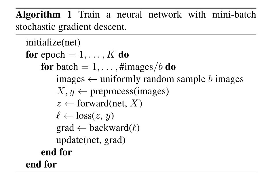
利用随机梯度下降的方法来训练神经网络的基本流程如下所示，首先先对于baseline情况的超参数进行一个假定，之后再讨论优化的方法：

Efficient Training

使用更低的精度和更大的batch size可以使得训练更加高效，这里提供了一系列这样的方法，有的可以同时提升准确率和训练速度。

Large-batch training

使用更大的batch size可能会减慢训练进程。对于凸优化问题，随着batch size的上升，收敛速率会下降，在神经网络当中也有相同的情况。在同样数目的epoch情况下，用大的batch训练的模型在验证集上的效果会更差。

下面有四个启发式的方法用来解决上面提到的问题：

Linear scaling learning rate

理论上来说，从估计梯度的角度，提升batch size并不会使得得到梯度的大小期望改变，而是使得它的方差更小。所以可以对于学习率进行成比率的缩放，能够使得效果提升。

比如在当batch size为256的时候，选用0.1的学习率。

那么当采用一个更大的batch size，例如$b$的时候，就将学习率设置为$0.1\times b/256$。

Learning rate warmup

在训练开始的时候，所有参数都是随机设置的，离最终结果可能会非常远，所以采用一个较大的学习率会导致数值上的不稳定，所以可以考虑在最开始使用一个很小的学习率，再慢慢地在训练较为稳定的时候切换到初始学习率。

例如，如果我们采用前$m$个batch来进行warm up的话，并且学习率的初值为$\eta$，那么在第$i$个batch，$1\le i \le m$，就选用大小为$i\eta/m$的学习率。

Zero $\gamma$

ResNet是有很多个residual block堆叠出来的，每个residual block的结果可以看成是$x+block(x)$，而block的最后一层通常是BN层，他会首先进行一个standardize，得到$\hat{x}$，然后在进行一个缩放$\gamma \hat{x}+\beta$，其中$\gamma$和$\beta$都是可学习的参数，通常被初始化为1和0。

可以考虑在初始化的时候，将所有的参数$\gamma$都设置成0，这样网络的输出就和他的输入相同，这样可以缩小网络，使得在最开始的时候训练变得更简单。

No bias decay

weight decay通常被用于所有可学习的参数来防止正则化，这里的trick就是只作用于权重，而不对bias包括BN层当中的$\gamma$和$\beta$做decay。

Low-precision training

通常是采用FP32来进行训练的，但是大量的TPU在FP16上面的效率会高很多，所以可以考虑采用FP16来进行训练，能够达到几倍的加速。

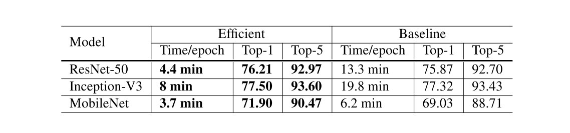
实验结果如上，其中Baseline的设置为$BS=256$，采用FP32，Efficient的设置为$BS=1024$，采用FP16。

Model Tweaks

原本的ResNet网络结构如图所示：

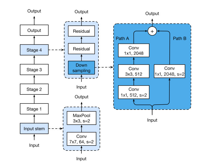
这里不多做介绍，文章提出了三种针对ResNet修改方式，分别记作ResNet-B/C/D，能够得到一定程度上的准确率提升。

ResNet-B

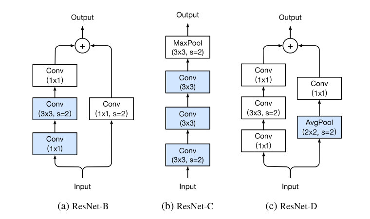
第一个所做的就是改变了downsampling的方式，由于如果采用$1\times 1$卷积同时选择stride为2的话，会丢失$3/4$的信息，这里在$3\times 3$的的卷积层来downsampling，理论上所有信息都会被接受到。

ResNet-C

一个发现就是卷积计算量随卷积核大小变化是二次多项式级别的，所以利用三层$3\times 3$的卷积来替代$7\times 7$的卷积层。

ResNet-D

从ResNet-B的角度更进一步，旁路也同样会有信息丢失的问题，所以将一层的$1 \times 1$卷积修改成一层Average Pooling再加上一层卷积，减少信息的丢失。

Experiment Result

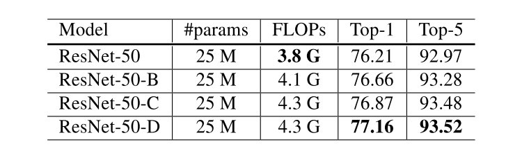
可以看到三者对于原始的ResNet结构准确率都有一定程度上的上升。

Training Refinements

Cosine Learning Rate Decay

采用最广泛的策略是指数衰减。这里提供的一种方法是利用cosine函数进行衰减，忽略掉最开始进行warmup的部分，假设一共有$T$个batch，那么在第$t$个batch上，学习率为：

$\eta_t = \frac{1}{2}(1+\cos(\frac{t\pi}{T}))\eta$

其中$\eta$就是初始的学习率，对比结果如下：

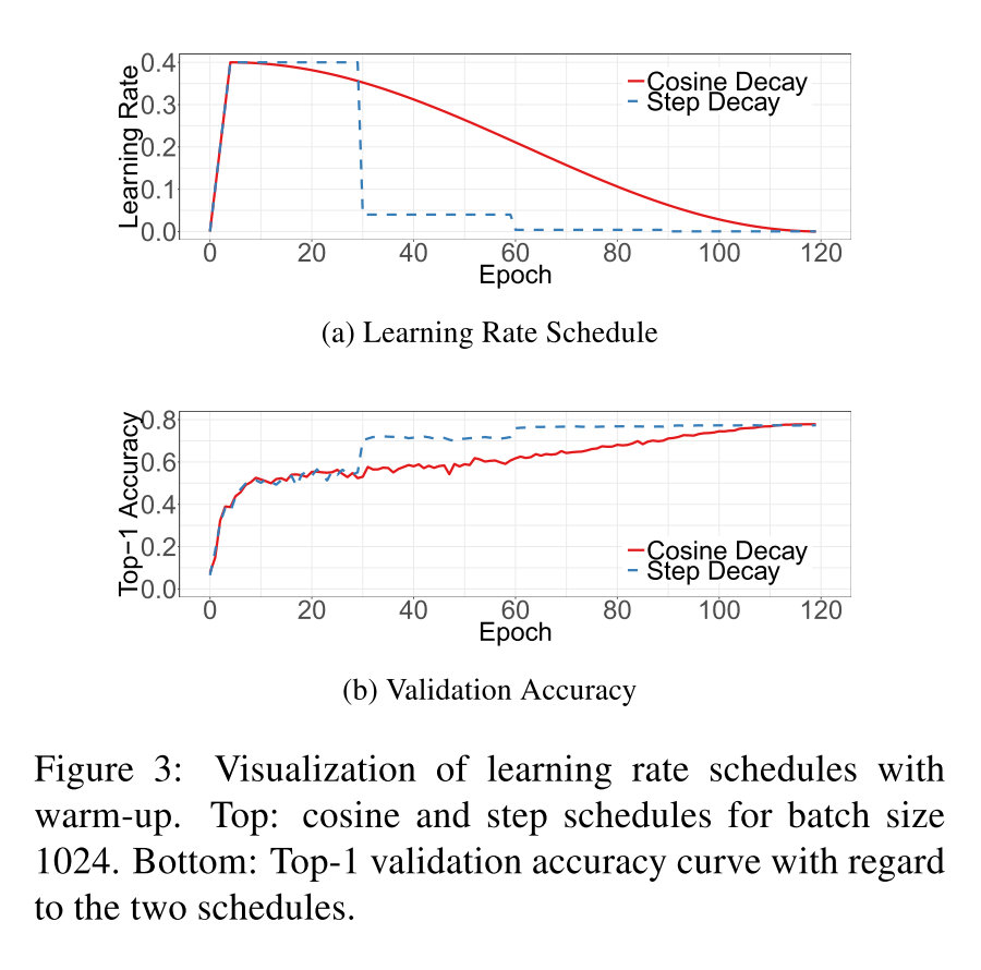
可以看到cosine decay在一开始和最终学习率下降的比较慢，在中间接近于线性的衰减。

Label Smoothing

对于分类任务，最后一层通常都是通过一个softmax函数来得到预测的概率，对于第$i$类的结果$q_i$：

$q_i = \frac{\exp(z_i)}{\sum_{j=1}^K \exp(z_j)}$

我们在学习过程当中最小化的是负的cross entropy：

$l(p,q) = -\sum_{i=1}^K p_i \log q_i$

$p_i$只有当$i=y$的时候为1，其余时候为0，于是就等价于：

$l(p,q) = -\log(q_y) = -z_y + \log (\sum_{i=1}^K \exp(z_i))$

要达到最小化的效果应当有$z_y^\star=\inf$，同时使得其他种类的$z_i$尽可能小，换言之，这样会倾向于让预测结果趋于极端值，最终导致overfit。

label smoothing的思想就是将真实概率构造为：

$p_i = \begin{cases}1-\epsilon &i=y\\\epsilon / (K-1) & \text{otherwise}\end{cases}$

其中$\epsilon$是一个小的常量，此时的最优解为：

$z_i^\star = \begin{cases}\log((K-1)(1-\epsilon)/\epsilon)+\alpha & i=y\\\alpha & \text{otherwise}\end{cases}$

其中$\alpha$是一个实数，这会使得最终全连接层的输出会趋向于一个有限值，能够更好地泛化。

里面$\log((K-1)(1-\epsilon)/\epsilon)$的部分就是正确分类和错误分类之间的gap，它随着$\epsilon$的增大不断缩小，当$\epsilon = (K-1)/K$的时候，实际上就是均匀分布，gap就为0了。

关于gap的可视化如下：

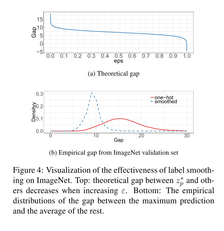
可以发现smooth之后gap总体均值变小，并且大gap的极端值情况有效减少了。

Knowledge Distillation

知识蒸馏中，我们尝试用一个学生模型来学习高准确率的老师模型里面的知识。方法就是利用一个distillation loss来惩罚学生模型偏离老师模型的预测概率。利用$p$作为真实概率，$z$和$r$分别作为学生网络和老师网络全连接层的输出，利用负的cross entropy作为loss，总的loss可以写成：

$l(p,\text{softmax}(z)) + T^2l(\text{softmax}(r/T),\text{softmax}(z/T))$

其中$T$为温度超参数，使得softmax函数的输出变得更为平滑。

Mixup Training

作为一个数据增强的手段，每次随机选择两个样本$(x_i,y_i)$和$(x_j,y_j)$。然后对两个样本加权来作为新的样本：

$\begin{aligned} \hat{x} &= \lambda x_i + (1-\lambda)x_j \\ \hat{y} &= \lambda y_i + (1-\lambda)y_j \end{aligned}$

其中$\lambda \in [0,1]$是一个从$\text{Beta}(\alpha,\alpha)$中采样出来的数，在mixup中只对于新的样本$(\hat{x},\hat{y})$来进行训练。

原文

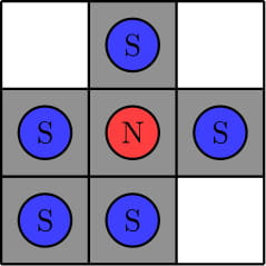
A monopole magnet is a magnet that only has one pole, either north or south. They don’t actually exist since real magnets have two poles, but this is a programming contest problem, so we don’t care.

There is an $n\times m$ grid. Initially, you may place some north magnets and some south magnets into the cells. You are allowed to place as many magnets as you like, even multiple in the same cell.

An operation is performed as follows. Choose a north magnet and a south magnet to activate. If they are in the same row or the same column and they occupy different cells, then the north magnet moves one unit closer to the south magnet. Otherwise, if they occupy the same cell or do not share a row or column, then nothing changes. Note that the south magnets are immovable.

Each cell of the grid is colored black or white. Let’s consider ways to place magnets in the cells so that the following conditions are met.

1. There is at least one south magnet in every row and every column.
2. If a cell is colored black, then it is possible for a north magnet to occupy this cell after some sequence of operations from the initial placement.
3. If a cell is colored white, then it is impossible for a north magnet to occupy this cell after some sequence of operations from the initial placement.

Determine if it is possible to place magnets such that these conditions are met. If it is possible, find the minimum number of north magnets required (there are no requirements on the number of south magnets).

Input

The first line contains two integers $n$ and $m$ ($1\le n,m\le 1000$) — the number of rows and the number of columns, respectively.

The next $n$ lines describe the coloring. The $i$-th of these lines contains a string of length $m$, where the $j$-th character denotes the color of the cell in row $i$ and column $j$. The characters “#” and “.” represent black and white, respectively. It is guaranteed, that the string will not contain any other characters.

Output

Output a single integer, the minimum possible number of north magnets required.

If there is no placement of magnets that satisfies all conditions, print a single integer −1.

Examples

input

1
2
3
4

3 3
.#.
###
##.

output

1

1

input

1
2
3
4
5

4 2
##
.#
.#
##

output

1

-1

input

1
2
3
4
5

4 5
....#
####.
.###.
.#...

output

1

2

input

1
2
3

2 1
.
#

output

1

-1

input

1
2
3
4

3 5
.....
.....
.....

output

1

0

Note

In the first test, here is an example placement of magnets:

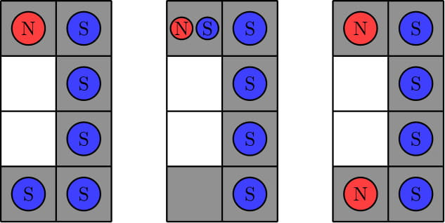
In the second test, we can show that no required placement of magnets exists. Here are three example placements that fail to meet the requirements. The first example violates rule 3 since we can move the north magnet down onto a white square. The second example violates rule 2 since we cannot move the north magnet to the bottom-left black square by any sequence of operations. The third example violates rule 1 since there is no south magnet in the first column.

In the third test, here is an example placement of magnets. We can show that there is no required placement of magnets with fewer north magnets.

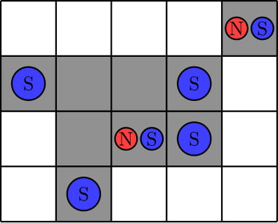
In the fourth test, we can show that no required placement of magnets exists. Here are two example placements that fail to meet the requirements. The first example violates rule 1 since there is no south magnet in the first row. The second example violates rules 1 and 3 since there is no south magnet in the second row and we can move the north magnet up one unit onto a white square.

In the fifth test, we can put the south magnet in each cell and no north magnets. Because there are no black cells, it will be a correct placement.

题意

有S和N两种磁铁，可以互相吸引，每次可以选择一个S和一个N激活，使得N向S方向移动，问需要有多少N磁铁可以满足（不限制S磁铁的数量）

• 每一行列都存在S磁铁
• 所有黑色区域都能够被N磁铁到达
• 所有白色区域都不可能被N磁铁到达

如果无法满足以上三条规则，那么就输出-1。

思路

首先排除所有不可能满足的情况：

1. 一行/一列有两段黑色区域，如果可以到达必定有S磁铁吸引，那么两段中间的白色区域就是可达的。所以每一行列必定只有一段黑色区域或全白。
2. 全白行但是没有全白列（行列对换相同），如果存在的话，由于每一行需要有S磁铁，而S磁铁放置的列是有黑色区域的，如果N磁铁到达该黑色区域，然后激活空白行处的S磁铁，会导致白色区域可达。

综上，放置磁铁的方式为将S磁铁放置在所有黑色块中和空白行列相交处。

N磁铁需要每一个连通区域放置一个，由于N磁铁不能跨区域移动，所以这种放置方式是最优的。

代码

1
2
3
4
5
6
7
8
9
10
11
12
13
14
15
16
17
18
19
20
21
22
23
24
25
26
27
28
29
30
31
32
33
34
35
36
37
38
39
40
41
42
43
44
45
46
47
48
49
50
51
52
53
54
55
56
57
58
59
60
61
62
63
64
65
66
67
68
69
70
71
72
73
74
75
76
77
78
79
80
81
82
83
84
85
86
87
88
89

#include <bits/stdc++.h>
using namespace std;

#define ll long long
#define maxn 1010

char grid[maxn][maxn];
bool unused_row;
bool unused_col;
bool vis[maxn][maxn]; 
int dir[4][2] = {{-1,0},{1,0},{0,1},{0,-1}};
int n,m;

void bfs(int i, int j){
    queue<pair<int,int>> q;
    vis[i][j] = true;
    q.push(make_pair(i,j));
    while(!q.empty()){
        auto temp = q.front();
        i = temp.first;
        j = temp.second;
        q.pop();
        for(int k=0;k<4;++k){
            int ii = i + dir[k][0];
            int jj = j + dir[k][1];
            if(ii>=0 && jj>=0 && ii<n &&jj<m && grid[ii][jj] == '#' && !vis[ii][jj]){
                vis[ii][jj] = true;
                q.push(make_pair(ii,jj));
            }
        }
    }
}

int main(){
    ios::sync_with_stdio(0);
    cin.tie(0);
    cout.tie(0);

    cin>>n>>m;
    for(int i=0;i<n;++i)
        cin>>grid[i];

    for(int i=0;i<n;++i){
        int cnt = 0;
        if(grid[i][0] == '#')
            cnt = 1;
        for(int j=1;j<m;++j)
            if(grid[i][j] == '#' && grid[i][j-1] == '.')
                ++cnt;
        if(cnt > 1){
            cout<<"-1"<<endl;
            return 0;
        }
        if(cnt == 0){
            unused_row = true;
        }
    }

    for(int j=0;j<m;++j){
        int cnt = 0;
        if(grid[0][j] == '#')
            cnt = 1;
        for(int i=1;i<n;++i)
            if(grid[i][j] == '#' && grid[i-1][j] == '.')
                ++cnt;
        if(cnt > 1){
            cout<<"-1"<<endl;
            return 0;
        }
        if(cnt == 0)
            unused_col = true;
    }
  
    if(unused_row ^ unused_col){
        cout<<"-1"<<endl;
        return 0;
    }

    int cnt = 0;
    for(int i=0;i<n;++i){
        for(int j=0;j<m;++j){
            if(grid[i][j] == '#' && !vis[i][j]){
                ++cnt;
                bfs(i,j);
            }
        }
    }
    cout<<cnt<<endl;
}

原文

Calculate the number of ways to place $n$ rooks on $n\times n$ chessboard so that both following conditions are met:

• each empty cell is under attack;
• exactly $k$ pairs of rooks attack each other.

An empty cell is under attack if there is at least one rook in the same row or at least one rook in the same column. Two rooks attack each other if they share the same row or column, and there are no other rooks between them. For example, there are only two pairs of rooks that attack each other in the following picture:

One of the ways to place the rooks for $n=3$ and $k=2$

Two ways to place the rooks are considered different if there exists at least one cell which is empty in one of the ways but contains a rook in another way.

The answer might be large, so print it modulo 998244353.

Input

The only line of the input contains two integers $n$ and $k$ ($1\le n\le 200000$; $0\le k\le\frac{n(n-1)}{2}$).

Output

Print one integer — the number of ways to place the rooks, taken modulo 998244353.

Examples

input

1

3 2

output

1

6

input

1

3 3

output

1

0

input

1

4 0

output

1

24

input

1

1337 42

output

1

807905441

题意

rook可以对同一行和同一列攻击，提供两个数$n$和$k$，求在$n\times n$的棋盘上放置$n$个rook使得：

• 所有棋盘格都可以被攻击到
• 有$k$对rook可以互相供给

的放置方法总数。

思路

由于所有地方都需要被攻击到，那么就相当于一定是每个行都有一个rook或者每个列都有一个rook.本质上是一个排列组合问题，可以发现，行和列实际上是对称的，所以只需要考虑行列当中的一种。

假设每个行上都有一个rook，如果$k\ne0$，那么必然是$n$个rook分布在$n-k$个列上。对应的排列方法一共有：

$(n-k)^n - C_{n-k}^{n-k-1}(n-k-1)^n+C_{n-k}^{n-k-2}(n-k-2)^n=\sum_{i=0}^{n-k}(-1)^i C_{n-k}^{i}(n-k-i)^n$

从上面的分析也可以发现，如果$k\ge n$，那么不存在符合的情况。再注意当$k\ne0$的时候需要，需要乘2，而$k=0$的时候直接作为结果就可以了。

代码

1
2
3
4
5
6
7
8
9
10
11
12
13
14
15
16
17
18
19
20
21
22
23
24
25
26
27
28
29
30
31
32
33
34
35
36
37
38
39
40
41
42
43
44
45
46
47
48
49
50
51
52
53
54
55
56
57
58
59
60
61
62

#include <bits/stdc++.h>
using namespace std;

#define ll long long
#define MOD 998244353

#define add(x,y) ((x+y)%MOD)
#define mul(x,y) ((x*y)%MOD)
#define sub(x,y) ((MOD+x-y)%MOD)

ll fastpow(ll x, ll y){
    ll temp = 1;
    while(y){
        if(y&1)
            temp = mul(temp, x);
        x = mul(x, x);
        y>>=1;
    }
    return temp;
}

ll inv(ll x){
    return fastpow(x,MOD-2);
}

ll frac[200100];

ll C(ll n, ll i){
    return mul(frac[n], inv(mul(frac[i], frac[n-i])));
}

int main(){
    ios::sync_with_stdio(0);
    cin.tie(0);
    cout.tie(0);

    int n,k;
    cin>>n>>k;
    
    if(k>=n){
        cout<<0<<endl;
        return 0;
    }

    ll ans = 0;
    frac[0] = 1;
    for(int i=1;i<=n;++i){
        frac[i] = mul(i, frac[i-1]);
    }
    for(int i=0;i<=n-k;++i){
        ll temp = mul(C(n-k,i), fastpow(n-k-i,n));
        if(i&1)
            ans = sub(ans, temp);
        else
            ans = add(ans,temp);
    }

    ans = mul(ans, C(n, n-k));
    if(k)
        ans = mul(ans, 2);
    cout<<ans<<endl;
}

Exercise 1

这个建立映射的函数实际上和kern/pmap.c当中的boot_alloc()存在类似的地方，都是利用一个静态的变量来保存当前分配空间的起始地方，然后不断的增长进行分配。由于base每次都会增长，所以每次都是映射新的页面。

1
2
3
4
5
6
7
8
9
10
11
12
13
14
15
16
17
18
19
20
21
22
23
24
25
26
27
28
29
30
31
32
33
34
35
36
37
38
39
40
41

//
// Reserve size bytes in the MMIO region and map [pa,pa+size) at this
// location.  Return the base of the reserved region.  size does *not*
// have to be multiple of PGSIZE.
//
void *
mmio_map_region(physaddr_t pa, size_t size)
{
	// Where to start the next region.  Initially, this is the
	// beginning of the MMIO region.  Because this is static, its
	// value will be preserved between calls to mmio_map_region
	// (just like nextfree in boot_alloc).
	static uintptr_t base = MMIOBASE;

	uintptr_t result;

	// Reserve size bytes of virtual memory starting at base and
	// map physical pages [pa,pa+size) to virtual addresses
	// [base,base+size).  Since this is device memory and not
	// regular DRAM, you'll have to tell the CPU that it isn't
	// safe to cache access to this memory.  Luckily, the page
	// tables provide bits for this purpose; simply create the
	// mapping with PTE_PCD|PTE_PWT (cache-disable and
	// write-through) in addition to PTE_W.  (If you're interested
	// in more details on this, see section 10.5 of IA32 volume
	// 3A.)
	//
	// Be sure to round size up to a multiple of PGSIZE and to
	// handle if this reservation would overflow MMIOLIM (it's
	// okay to simply panic if this happens).
	//
	// Hint: The staff solution uses boot_map_region.
	//
	// Your code here:
	if(base + ROUNDUP(size, PGSIZE) >= MMIOLIM)
		panic("mmio_map_region: out of memory\n");
	boot_map_region(kern_pgdir, base, size, pa, PTE_PCD | PTE_PWT | PTE_W);
	result = base;
	base += ROUNDUP(size, PGSIZE);
	return (void *)result;
}

Exercise 2

修改page_init()的内容如下，只是增加一个特殊处理：

1
2
3
4
5
6
7
8
9
10
11
12
13
14
15
16
17

// case 1:
pages[0].pp_ref = 1;
pages[0].pp_link = NULL;
// case 2, 3, 4:
for (i = 1; i < npages; i++) {
	if((IOPHYSMEM <= i * PGSIZE && i * PGSIZE < pa_free_start) || page2pa(pages + i) == MPENTRY_PADDR)
	{
		pages[i].pp_ref = 1;
		pages[i].pp_link = NULL;
	}
	else
	{
		pages[i].pp_ref = 0;
		pages[i].pp_link = page_free_list;
		page_free_list = &pages[i];
	}
}

只要在第6行添加一个判断就可以了。

之后执行make qemu就可以看到如下的check都已经成功了。

1
2
3

check_page_free_list() succeeded!
check_page_alloc() succeeded!
check_page() succeeded!

Question 1

宏MPBOOTPHYS的作用是将高地址转换为低地址，使得可以在实模式下进行访问。在boot.S当中，本来就已经被链接到了低地址，不需要进行转换，而mpentry.S的代码都位于KERNBASE的上方，所以需要手动的利用MPBOOTPHYS宏进行转换。

Exercise 3

这里直接利用一个循环进行映射，由于每个栈之间是存在一个Gap的，所以只有[kstacktop_i - KSTKSIZE, kstacktop_i)部分需要进行映射。

1
2
3
4
5
6
7
8
9
10
11
12
13
14
15
16
17
18
19
20
21
22
23
24
25
26

// Modify mappings in kern_pgdir to support SMP
//   - Map the per-CPU stacks in the region [KSTACKTOP-PTSIZE, KSTACKTOP)
//
static void
mem_init_mp(void)
{
	// Map per-CPU stacks starting at KSTACKTOP, for up to 'NCPU' CPUs.
	//
	// For CPU i, use the physical memory that 'percpu_kstacks[i]' refers
	// to as its kernel stack. CPU i's kernel stack grows down from virtual
	// address kstacktop_i = KSTACKTOP - i * (KSTKSIZE + KSTKGAP), and is
	// divided into two pieces, just like the single stack you set up in
	// mem_init:
	//     * [kstacktop_i - KSTKSIZE, kstacktop_i)
	//          -- backed by physical memory
	//     * [kstacktop_i - (KSTKSIZE + KSTKGAP), kstacktop_i - KSTKSIZE)
	//          -- not backed; so if the kernel overflows its stack,
	//             it will fault rather than overwrite another CPU's stack.
	//             Known as a "guard page".
	//     Permissions: kernel RW, user NONE
	//
	// LAB 4: Your code here:
	uint32_t i, kstacktop_i;
	for(i=0, kstacktop_i=KSTACKTOP;i < NCPU; ++i, kstacktop_i -= KSTKSIZE + KSTKGAP)
		boot_map_region(kern_pgdir, kstacktop_i - KSTKSIZE, KSTKSIZE, PADDR(percpu_kstacks[i]), PTE_W);
}

Exercise 4

这里实际上就是用thiscpu来替换原本的全局变量，使得本来是在lab3当中对于单CPU适用的情况可以适用于多个CPU的情形。

1
2
3
4
5
6
7
8
9
10
11
12
13
14
15
16
17
18
19
20
21
22
23
24
25
26
27
28
29
30
31
32
33
34
35
36
37
38
39
40
41
42
43
44
45
46
47

// Initialize and load the per-CPU TSS and IDT
void
trap_init_percpu(void)
{
	// The example code here sets up the Task State Segment (TSS) and
	// the TSS descriptor for CPU 0. But it is incorrect if we are
	// running on other CPUs because each CPU has its own kernel stack.
	// Fix the code so that it works for all CPUs.
	//
	// Hints:
	//   - The macro "thiscpu" always refers to the current CPU's
	//     struct CpuInfo;
	//   - The ID of the current CPU is given by cpunum() or
	//     thiscpu->cpu_id;
	//   - Use "thiscpu->cpu_ts" as the TSS for the current CPU,
	//     rather than the global "ts" variable;
	//   - Use gdt[(GD_TSS0 >> 3) + i] for CPU i's TSS descriptor;
	//   - You mapped the per-CPU kernel stacks in mem_init_mp()
	//   - Initialize cpu_ts.ts_iomb to prevent unauthorized environments
	//     from doing IO (0 is not the correct value!)
	//
	// ltr sets a 'busy' flag in the TSS selector, so if you
	// accidentally load the same TSS on more than one CPU, you'll
	// get a triple fault.  If you set up an individual CPU's TSS
	// wrong, you may not get a fault until you try to return from
	// user space on that CPU.
	//
	// LAB 4: Your code here:

	// Setup a TSS so that we get the right stack
	// when we trap to the kernel.
	thiscpu->cpu_ts.ts_esp0 = KSTACKTOP - cpunum() * (KSTKSIZE + KSTKGAP);
	thiscpu->cpu_ts.ts_ss0 = GD_KD;
	thiscpu->cpu_ts.ts_iomb = sizeof(struct Taskstate);

	// Initialize the TSS slot of the gdt.
	gdt[(GD_TSS0 >> 3) + cpunum()] = SEG16(STS_T32A, (uint32_t) (&(thiscpu->cpu_ts)),
					sizeof(struct Taskstate) - 1, 0);
	gdt[(GD_TSS0 >> 3) + cpunum()].sd_s = 0;

	// Load the TSS selector (like other segment selectors, the
	// bottom three bits are special; we leave them 0)
	ltr(GD_TSS0 + (cpunum() << 3));

	// Load the IDT
	lidt(&idt_pd);
}

Exercise 5

根据文档的描述在四个所需要插入大内核锁的地方进行lock_kernel()和unlock_kernel()的操作。

• In i386_init(), acquire the lock before the BSP wakes up the other CPUs.

  1 2 3 4 5 6

  // Acquire the big kernel lock before waking up APs // Your code here: lock_kernel(); // Starting non-boot CPUs boot_aps();

• In mp_main(), acquire the lock after initializing the AP, and then call sched_yield() to start running environments on this AP.

  1 2 3 4 5 6 7

  // Now that we have finished some basic setup, call sched_yield() // to start running processes on this CPU. But make sure that // only one CPU can enter the scheduler at a time! // // Your code here: lock_kernel(); sched_yield();

• In trap(), acquire the lock when trapped from user mode. To determine whether a trap happened in user mode or in kernel mode, check the low bits of the tf_cs.

  1 2 3 4 5 6

  // Trapped from user mode. // Acquire the big kernel lock before doing any // serious kernel work. // LAB 4: Your code here. lock_kernel(); assert(curenv);

• In env_run(), release the lock right before switching to user mode. Do not do that too early or too late, otherwise you will experience races or deadlocks.

  1 2 3

  lcr3(PADDR(e->env_pgdir)); unlock_kernel(); env_pop_tf(&(e->env_tf));

Question 2

从trapentry.S当中可以看到，在调用trap()之前（还没有获得大内核锁），这个时候就已经往内核栈中压入了寄存器信息，如果内核栈不分离的话，在这个时候切换就会造成错误。

Exercise 6

这里的调度方法实际上是一个非常暴力的轮询，如果找到了一个状态是ENV_RUNNABLE的进程那么就让他上CPU。如果找了一圈都没有找到合适的进程的话，就看起始进程，如果它本来就在当前CPU上运行的话，那么就继续运行，否则的话一个进程不能在两个CPU上同时运行，就调用sched_halt()。

1
2
3
4
5
6
7
8
9
10
11
12
13
14
15
16
17
18
19
20
21
22
23
24
25
26
27
28
29
30
31
32
33
34
35

// Choose a user environment to run and run it.
void
sched_yield(void)
{
	struct Env *idle;

	// Implement simple round-robin scheduling.
	//
	// Search through 'envs' for an ENV_RUNNABLE environment in
	// circular fashion starting just after the env this CPU was
	// last running.  Switch to the first such environment found.
	//
	// If no envs are runnable, but the environment previously
	// running on this CPU is still ENV_RUNNING, it's okay to
	// choose that environment.
	//
	// Never choose an environment that's currently running on
	// another CPU (env_status == ENV_RUNNING). If there are
	// no runnable environments, simply drop through to the code
	// below to halt the cpu.

	// LAB 4: Your code here.
	int start_i, i;
	if(!curenv)
		start_i = 0;
	else
		start_i = curenv->env_id;
	for(i = 0; i < NENV; ++i)
		if(envs[(start_i + i)%NENV].env_status == ENV_RUNNABLE)
			env_run(&envs[(start_i + i)%NENV]);
	if(envs[start_i%NENV].env_status == ENV_RUNNING && envs[start_i%NENV].env_cpunum == cpunum())
		env_run(&envs[start_i%NENV]);
	// sched_halt never returns
	sched_halt();
}

在syscall()当中添加新的系统调用的分发：

1
2
3

case SYS_yield:
	sys_yield();
	return 0;

在mp_main()当中调用sched_yield()。

1
2
3
4
5
6
7
8
9
10
11
12
13
14
15
16
17
18
19
20
21
22
23
24

// Setup code for APs
void
mp_main(void)
{
	// We are in high EIP now, safe to switch to kern_pgdir 
	lcr3(PADDR(kern_pgdir));
	cprintf("SMP: CPU %d starting\n", cpunum());

	lapic_init();
	env_init_percpu();
	trap_init_percpu();
	xchg(&thiscpu->cpu_status, CPU_STARTED); // tell boot_aps() we're up

	// Now that we have finished some basic setup, call sched_yield()
	// to start running processes on this CPU.  But make sure that
	// only one CPU can enter the scheduler at a time!
	//
	// Your code here:
	lock_kernel();
	sched_yield();

	// Remove this after you finish Exercise 6
	for (;;);
}

Question 3

看env_run()当中对应代码部分如下：

1
2
3
4
5
6
7
8
9
10

if(curenv != NULL && curenv->env_status == ENV_RUNNING)
	curenv->env_status = ENV_RUNNABLE;
curenv = e;
e->env_status = ENV_RUNNING;
++(e->env_runs);
lcr3(PADDR(e->env_pgdir));

unlock_kernel();

env_pop_tf(&(e->env_tf));

在lcr3()前后都能够正常对e进行解引用是因为，在设置env_pgdir的时候是以kern_pgdir作为模板进行修改的，e地址在两个地址空间中是映射到同一个物理地址的，所以这里进行解引用的操作不会有问题。

Question 4

保存寄存器信息的操作发生在kern/trapentry.S当中：

1
2
3
4
5
6
7
8
9
10
11

.global _alltraps
_alltraps:
	pushl %ds
	pushl %es
	pushal
	pushl $GD_KD
	popl %ds
	pushl $GD_KD
	popl %es
	pushl %esp
	call trap

恢复寄存器的操作发生在kern/env.c的env_pop_tf()当中：

1
2
3
4
5
6
7
8
9
10
11
12
13
14
15
16